Quickstart: Access Data from Disc at DKRZ
Browsing the STAC catalog
We create a Client from the pystac_client package. For this example we assume, that we already know the collection ID and item ID. This allows us to navigate directly through the catalog.
Browsing the catalog is a topic for another guide.
To open the catalog, we need its base URL, here https://wwestac.cloud.dkrz.de/stac-fastapi-es/.
Using a different URL, grants access to a different catalog.
import pystac_client
catalog = pystac_client.Client.open("https://wwestac.cloud.dkrz.de/stac-fastapi-es/")
collection = catalog.get_collection("ngc3026")
items = asset = collection.get_items()
item = collection.get_item('ngc3026_P1D_7')
print(item)
<Item id=ngc3026_P1D_7>
Opening the Dataset
As the last step, we select an asset, in other words an way to open our desired dataset. Here, we select disk. Printing the path to would allow us using this path for the data analysis. Each item can have several assets with different options to open the desired dataset.
zarr_path=item.assets['disk'].href
print(zarr_path)
file:///work/bm1235/k203123/nextgems_cycle3/experiments/ngc3026/outdata/ngc3026_P1D_7.zarr
Now we can open the dataset and inspect it. The default output gives already several information on data axis, variables etc.
In this example we use the xarray package, which gives a common interface and supports a wide variety of file formats. xarray also gives extensive features for data processing.
For the usage, you need to install the python zarr package. The required import is handeled by xarray.
import xarray as xr
ds = xr.open_zarr(zarr_path)
ds
<xarray.Dataset>
Dimensions:                              (time: 370, depth_half: 129,
                                          cell: 196608, level_full: 90, crs: 1,
                                          depth_full: 128,
                                          soil_depth_water_level: 5,
                                          level_half: 91,
                                          soil_depth_energy_level: 5)
Coordinates:
  * crs                                  (crs) float32 nan
  * depth_full                           (depth_full) float32 1.0 ... 5.904e+03
  * depth_half                           (depth_half) float32 0.0 ... 6.003e+03
  * level_full                           (level_full) int32 1 2 3 4 ... 88 89 90
  * level_half                           (level_half) int32 1 2 3 4 ... 89 90 91
  * soil_depth_energy_level              (soil_depth_energy_level) float32 0....
  * soil_depth_water_level               (soil_depth_water_level) float32 0.0...
  * time                                 (time) datetime64[ns] 2020-01-21 ......
Dimensions without coordinates: cell
Data variables: (12/88)
    a_tracer_v_to                        (time, depth_half, cell) float32 dask.array<chunksize=(1, 33, 196608), meta=np.ndarray>
    atmos_fluxes_frshflux_evaporation    (time, cell) float32 dask.array<chunksize=(1, 196608), meta=np.ndarray>
    atmos_fluxes_frshflux_precipitation  (time, cell) float32 dask.array<chunksize=(1, 196608), meta=np.ndarray>
    atmos_fluxes_frshflux_runoff         (time, cell) float32 dask.array<chunksize=(1, 196608), meta=np.ndarray>
    atmos_fluxes_frshflux_snowfall       (time, cell) float32 dask.array<chunksize=(1, 196608), meta=np.ndarray>
    atmos_fluxes_heatflux_latent         (time, cell) float32 dask.array<chunksize=(1, 196608), meta=np.ndarray>
    ...                                   ...
    va                                   (time, level_full, cell) float32 dask.array<chunksize=(1, 30, 196608), meta=np.ndarray>
    vas                                  (time, cell) float32 dask.array<chunksize=(1, 196608), meta=np.ndarray>
    w                                    (time, depth_half, cell) float32 dask.array<chunksize=(1, 33, 196608), meta=np.ndarray>
    wa_phy                               (time, level_half, cell) float32 dask.array<chunksize=(1, 31, 196608), meta=np.ndarray>
    wind_speed_10m                       (time, cell) float32 dask.array<chunksize=(1, 196608), meta=np.ndarray>
zos (time, cell) float32 dask.array<chunksize=(1, 196608), meta=np.ndarray>- time: 370
- depth_half: 129
- cell: 196608
- level_full: 90
- crs: 1
- depth_full: 128
- soil_depth_water_level: 5
- level_half: 91
- soil_depth_energy_level: 5
- crs(crs)float32nan
- grid_mapping_name :
- healpix
- healpix_nside :
- 128
- healpix_order :
- nest
array([nan], dtype=float32)
- depth_full(depth_full)float321.0 3.05 5.2 ... 5.71e+03 5.904e+03
- axis :
- Z
- long_name :
- depth_below_sea
- positive :
- down
- standard_name :
- depth
- units :
- m
array([1.00000e+00, 3.05000e+00, 5.20000e+00, 7.45000e+00, 9.80000e+00, 1.22500e+01, 1.48000e+01, 1.74500e+01, 2.02000e+01, 2.31000e+01, 2.61500e+01, 2.93000e+01, 3.26000e+01, 3.60500e+01, 3.96500e+01, 4.34500e+01, 4.74000e+01, 5.15000e+01, 5.58000e+01, 6.03000e+01, 6.50000e+01, 6.99000e+01, 7.50500e+01, 8.04500e+01, 8.61000e+01, 9.20000e+01, 9.81500e+01, 1.04600e+02, 1.11350e+02, 1.18400e+02, 1.25750e+02, 1.33400e+02, 1.41400e+02, 1.49750e+02, 1.58450e+02, 1.67550e+02, 1.77100e+02, 1.87100e+02, 1.97550e+02, 2.08450e+02, 2.19750e+02, 2.31450e+02, 2.43550e+02, 2.56050e+02, 2.68950e+02, 2.82250e+02, 2.96000e+02, 3.10250e+02, 3.24950e+02, 3.40100e+02, 3.55750e+02, 3.71950e+02, 3.88700e+02, 4.06000e+02, 4.23900e+02, 4.42400e+02, 4.61500e+02, 4.81200e+02, 5.01550e+02, 5.22600e+02, 5.44350e+02, 5.66800e+02, 5.90000e+02, 6.14000e+02, 6.38800e+02, 6.64400e+02, 6.90850e+02, 7.18200e+02, 7.46450e+02, 7.75650e+02, 8.05800e+02, 8.36950e+02, 8.69150e+02, 9.02400e+02, 9.36750e+02, 9.72250e+02, 1.00895e+03, 1.04685e+03, 1.08600e+03, 1.12645e+03, 1.16825e+03, 1.21145e+03, 1.25605e+03, 1.30210e+03, 1.34970e+03, 1.39890e+03, 1.44975e+03, 1.50230e+03, 1.55660e+03, 1.61270e+03, 1.67065e+03, 1.73050e+03, 1.79235e+03, 1.85625e+03, 1.92225e+03, 1.99045e+03, 2.06090e+03, 2.13370e+03, 2.20895e+03, 2.28670e+03, 2.36700e+03, 2.44995e+03, 2.53565e+03, 2.62420e+03, 2.71570e+03, 2.81025e+03, 2.90795e+03, 3.00890e+03, 3.11320e+03, 3.22095e+03, 3.33230e+03, 3.44735e+03, 3.56620e+03, 3.68900e+03, 3.81585e+03, 3.94690e+03, 4.08230e+03, 4.22220e+03, 4.36675e+03, 4.51610e+03, 4.67045e+03, 4.82995e+03, 4.99470e+03, 5.16490e+03, 5.34075e+03, 5.52245e+03, 5.71020e+03, 5.90415e+03], dtype=float32) - depth_half(depth_half)float320.0 2.0 4.1 ... 5.806e+03 6.003e+03
- axis :
- Z
- long_name :
- depth_below_sea
- positive :
- down
- standard_name :
- depth
- units :
- m
array([0.0000e+00, 2.0000e+00, 4.1000e+00, 6.3000e+00, 8.6000e+00, 1.1000e+01, 1.3500e+01, 1.6100e+01, 1.8800e+01, 2.1600e+01, 2.4600e+01, 2.7700e+01, 3.0900e+01, 3.4300e+01, 3.7800e+01, 4.1500e+01, 4.5400e+01, 4.9400e+01, 5.3600e+01, 5.8000e+01, 6.2600e+01, 6.7400e+01, 7.2400e+01, 7.7700e+01, 8.3200e+01, 8.9000e+01, 9.5000e+01, 1.0130e+02, 1.0790e+02, 1.1480e+02, 1.2200e+02, 1.2950e+02, 1.3730e+02, 1.4550e+02, 1.5400e+02, 1.6290e+02, 1.7220e+02, 1.8200e+02, 1.9220e+02, 2.0290e+02, 2.1400e+02, 2.2550e+02, 2.3740e+02, 2.4970e+02, 2.6240e+02, 2.7550e+02, 2.8900e+02, 3.0300e+02, 3.1750e+02, 3.3240e+02, 3.4780e+02, 3.6370e+02, 3.8020e+02, 3.9720e+02, 4.1480e+02, 4.3300e+02, 4.5180e+02, 4.7120e+02, 4.9120e+02, 5.1190e+02, 5.3330e+02, 5.5540e+02, 5.7820e+02, 6.0180e+02, 6.2620e+02, 6.5140e+02, 6.7740e+02, 7.0430e+02, 7.3210e+02, 7.6080e+02, 7.9050e+02, 8.2110e+02, 8.5280e+02, 8.8550e+02, 9.1930e+02, 9.5420e+02, 9.9030e+02, 1.0276e+03, 1.0661e+03, 1.1059e+03, 1.1470e+03, 1.1895e+03, 1.2334e+03, 1.2787e+03, 1.3255e+03, 1.3739e+03, 1.4239e+03, 1.4756e+03, 1.5290e+03, 1.5842e+03, 1.6412e+03, 1.7001e+03, 1.7609e+03, 1.8238e+03, 1.8887e+03, 1.9558e+03, 2.0251e+03, 2.0967e+03, 2.1707e+03, 2.2472e+03, 2.3262e+03, 2.4078e+03, 2.4921e+03, 2.5792e+03, 2.6692e+03, 2.7622e+03, 2.8583e+03, 2.9576e+03, 3.0602e+03, 3.1662e+03, 3.2757e+03, 3.3889e+03, 3.5058e+03, 3.6266e+03, 3.7514e+03, 3.8803e+03, 4.0135e+03, 4.1511e+03, 4.2933e+03, 4.4402e+03, 4.5920e+03, 4.7489e+03, 4.9110e+03, 5.0784e+03, 5.2514e+03, 5.4301e+03, 5.6148e+03, 5.8056e+03, 6.0027e+03], dtype=float32) - level_full(level_full)int321 2 3 4 5 6 7 ... 85 86 87 88 89 90
- axis :
- Z
- long_name :
- generalized_height
- positive :
- down
- standard_name :
- height
array([ 1, 2, 3, 4, 5, 6, 7, 8, 9, 10, 11, 12, 13, 14, 15, 16, 17, 18, 19, 20, 21, 22, 23, 24, 25, 26, 27, 28, 29, 30, 31, 32, 33, 34, 35, 36, 37, 38, 39, 40, 41, 42, 43, 44, 45, 46, 47, 48, 49, 50, 51, 52, 53, 54, 55, 56, 57, 58, 59, 60, 61, 62, 63, 64, 65, 66, 67, 68, 69, 70, 71, 72, 73, 74, 75, 76, 77, 78, 79, 80, 81, 82, 83, 84, 85, 86, 87, 88, 89, 90], dtype=int32) - level_half(level_half)int321 2 3 4 5 6 7 ... 86 87 88 89 90 91
- axis :
- Z
- long_name :
- generalized_height
- positive :
- down
- standard_name :
- height
array([ 1, 2, 3, 4, 5, 6, 7, 8, 9, 10, 11, 12, 13, 14, 15, 16, 17, 18, 19, 20, 21, 22, 23, 24, 25, 26, 27, 28, 29, 30, 31, 32, 33, 34, 35, 36, 37, 38, 39, 40, 41, 42, 43, 44, 45, 46, 47, 48, 49, 50, 51, 52, 53, 54, 55, 56, 57, 58, 59, 60, 61, 62, 63, 64, 65, 66, 67, 68, 69, 70, 71, 72, 73, 74, 75, 76, 77, 78, 79, 80, 81, 82, 83, 84, 85, 86, 87, 88, 89, 90, 91], dtype=int32) - soil_depth_energy_level(soil_depth_energy_level)float320.0325 0.192 0.7755 2.683 6.984
- axis :
- Z
- long_name :
- depth_below_land
- positive :
- down
- units :
- m
array([0.0325, 0.192 , 0.7755, 2.683 , 6.984 ], dtype=float32)
- soil_depth_water_level(soil_depth_water_level)float320.0325 0.192 0.7755 2.683 6.984
- axis :
- Z
- long_name :
- depth_below_land
- positive :
- down
- units :
- m
array([0.0325, 0.192 , 0.7755, 2.683 , 6.984 ], dtype=float32)
- time(time)datetime64[ns]2020-01-21 ... 2021-01-24
- axis :
- T
array(['2020-01-21T00:00:00.000000000', '2020-01-22T00:00:00.000000000',
       '2020-01-23T00:00:00.000000000', ..., '2021-01-22T00:00:00.000000000',
       '2021-01-23T00:00:00.000000000', '2021-01-24T00:00:00.000000000'],
      dtype='datetime64[ns]')
- a_tracer_v_to(time, depth_half, cell)float32dask.array<chunksize=(1, 33, 196608), meta=np.ndarray>
- cell_methods :
- time: mean cell: mean
- component :
- ocean
- grid_mapping :
- crs
- long_name :
- sea water vertical diffusivity
- standard_name :
- ocean_vertical_diffusivity
- units :
- m2 s-1
- vgrid :
- depth_below_sea_half
Array Chunk Bytes 34.96 GiB 24.75 MiB Shape (370, 129, 196608) (1, 33, 196608) Dask graph 1480 chunks in 2 graph layers Data type float32 numpy.ndarray - atmos_fluxes_frshflux_evaporation(time, cell)float32dask.array<chunksize=(1, 196608), meta=np.ndarray>
- cell_methods :
- time: mean cell: mean
- component :
- ocean
- grid_mapping :
- crs
- units :
- m/s
- vgrid :
- surface
Array Chunk Bytes 277.50 MiB 768.00 kiB Shape (370, 196608) (1, 196608) Dask graph 370 chunks in 2 graph layers Data type float32 numpy.ndarray - atmos_fluxes_frshflux_precipitation(time, cell)float32dask.array<chunksize=(1, 196608), meta=np.ndarray>
- cell_methods :
- time: mean cell: mean
- component :
- ocean
- grid_mapping :
- crs
- units :
- m/s
- vgrid :
- surface
Array Chunk Bytes 277.50 MiB 768.00 kiB Shape (370, 196608) (1, 196608) Dask graph 370 chunks in 2 graph layers Data type float32 numpy.ndarray - atmos_fluxes_frshflux_runoff(time, cell)float32dask.array<chunksize=(1, 196608), meta=np.ndarray>
- cell_methods :
- time: mean cell: mean
- component :
- ocean
- grid_mapping :
- crs
- units :
- m/s
- vgrid :
- surface
Array Chunk Bytes 277.50 MiB 768.00 kiB Shape (370, 196608) (1, 196608) Dask graph 370 chunks in 2 graph layers Data type float32 numpy.ndarray - atmos_fluxes_frshflux_snowfall(time, cell)float32dask.array<chunksize=(1, 196608), meta=np.ndarray>
- cell_methods :
- time: mean cell: mean
- component :
- ocean
- grid_mapping :
- crs
- units :
- m/s
- vgrid :
- surface
Array Chunk Bytes 277.50 MiB 768.00 kiB Shape (370, 196608) (1, 196608) Dask graph 370 chunks in 2 graph layers Data type float32 numpy.ndarray - atmos_fluxes_heatflux_latent(time, cell)float32dask.array<chunksize=(1, 196608), meta=np.ndarray>
- cell_methods :
- time: mean cell: mean
- component :
- ocean
- grid_mapping :
- crs
- units :
- W/m2
- vgrid :
- surface
Array Chunk Bytes 277.50 MiB 768.00 kiB Shape (370, 196608) (1, 196608) Dask graph 370 chunks in 2 graph layers Data type float32 numpy.ndarray - atmos_fluxes_heatflux_longwave(time, cell)float32dask.array<chunksize=(1, 196608), meta=np.ndarray>
- cell_methods :
- time: mean cell: mean
- component :
- ocean
- grid_mapping :
- crs
- units :
- W/m2
- vgrid :
- surface
Array Chunk Bytes 277.50 MiB 768.00 kiB Shape (370, 196608) (1, 196608) Dask graph 370 chunks in 2 graph layers Data type float32 numpy.ndarray - atmos_fluxes_heatflux_sensible(time, cell)float32dask.array<chunksize=(1, 196608), meta=np.ndarray>
- cell_methods :
- time: mean cell: mean
- component :
- ocean
- grid_mapping :
- crs
- units :
- W/m2
- vgrid :
- surface
Array Chunk Bytes 277.50 MiB 768.00 kiB Shape (370, 196608) (1, 196608) Dask graph 370 chunks in 2 graph layers Data type float32 numpy.ndarray - atmos_fluxes_heatflux_shortwave(time, cell)float32dask.array<chunksize=(1, 196608), meta=np.ndarray>
- cell_methods :
- time: mean cell: mean
- component :
- ocean
- grid_mapping :
- crs
- units :
- W/m2
- vgrid :
- surface
Array Chunk Bytes 277.50 MiB 768.00 kiB Shape (370, 196608) (1, 196608) Dask graph 370 chunks in 2 graph layers Data type float32 numpy.ndarray - atmos_fluxes_heatflux_total(time, cell)float32dask.array<chunksize=(1, 196608), meta=np.ndarray>
- cell_methods :
- time: mean cell: mean
- component :
- ocean
- grid_mapping :
- crs
- units :
- W/m2
- vgrid :
- surface
Array Chunk Bytes 277.50 MiB 768.00 kiB Shape (370, 196608) (1, 196608) Dask graph 370 chunks in 2 graph layers Data type float32 numpy.ndarray - atmos_fluxes_stress_x(time, cell)float32dask.array<chunksize=(1, 196608), meta=np.ndarray>
- cell_methods :
- time: mean cell: mean
- component :
- ocean
- grid_mapping :
- crs
- units :
- Pa
- vgrid :
- surface
Array Chunk Bytes 277.50 MiB 768.00 kiB Shape (370, 196608) (1, 196608) Dask graph 370 chunks in 2 graph layers Data type float32 numpy.ndarray - atmos_fluxes_stress_xw(time, cell)float32dask.array<chunksize=(1, 196608), meta=np.ndarray>
- cell_methods :
- time: mean cell: mean
- component :
- ocean
- grid_mapping :
- crs
- units :
- Pa
- vgrid :
- surface
Array Chunk Bytes 277.50 MiB 768.00 kiB Shape (370, 196608) (1, 196608) Dask graph 370 chunks in 2 graph layers Data type float32 numpy.ndarray - atmos_fluxes_stress_y(time, cell)float32dask.array<chunksize=(1, 196608), meta=np.ndarray>
- cell_methods :
- time: mean cell: mean
- component :
- ocean
- grid_mapping :
- crs
- units :
- Pa
- vgrid :
- surface
Array Chunk Bytes 277.50 MiB 768.00 kiB Shape (370, 196608) (1, 196608) Dask graph 370 chunks in 2 graph layers Data type float32 numpy.ndarray - atmos_fluxes_stress_yw(time, cell)float32dask.array<chunksize=(1, 196608), meta=np.ndarray>
- cell_methods :
- time: mean cell: mean
- component :
- ocean
- grid_mapping :
- crs
- units :
- Pa
- vgrid :
- surface
Array Chunk Bytes 277.50 MiB 768.00 kiB Shape (370, 196608) (1, 196608) Dask graph 370 chunks in 2 graph layers Data type float32 numpy.ndarray - cli(time, level_full, cell)float32dask.array<chunksize=(1, 30, 196608), meta=np.ndarray>
- cell_methods :
- time: mean cell: mean
- component :
- atmo
- grid_mapping :
- crs
- long_name :
- specific cloud ice content
- units :
- kg kg-1
- vgrid :
- reference
Array Chunk Bytes 24.39 GiB 22.50 MiB Shape (370, 90, 196608) (1, 30, 196608) Dask graph 1110 chunks in 2 graph layers Data type float32 numpy.ndarray - clivi(time, cell)float32dask.array<chunksize=(1, 196608), meta=np.ndarray>
- cell_methods :
- time: mean cell: mean
- component :
- atmo
- grid_mapping :
- crs
- long_name :
- vertically integrated cloud ice
- units :
- kg m-2
- vgrid :
- atmosphere
Array Chunk Bytes 277.50 MiB 768.00 kiB Shape (370, 196608) (1, 196608) Dask graph 370 chunks in 2 graph layers Data type float32 numpy.ndarray - cllvi(time, cell)float32dask.array<chunksize=(1, 196608), meta=np.ndarray>
- cell_methods :
- time: mean cell: mean
- component :
- atmo
- grid_mapping :
- crs
- long_name :
- vertically integrated cloud water
- units :
- kg m-2
- vgrid :
- atmosphere
Array Chunk Bytes 277.50 MiB 768.00 kiB Shape (370, 196608) (1, 196608) Dask graph 370 chunks in 2 graph layers Data type float32 numpy.ndarray - clw(time, level_full, cell)float32dask.array<chunksize=(1, 30, 196608), meta=np.ndarray>
- cell_methods :
- time: mean cell: mean
- component :
- atmo
- grid_mapping :
- crs
- long_name :
- specific cloud water content
- units :
- kg kg-1
- vgrid :
- reference
Array Chunk Bytes 24.39 GiB 22.50 MiB Shape (370, 90, 196608) (1, 30, 196608) Dask graph 1110 chunks in 2 graph layers Data type float32 numpy.ndarray - conc(time, cell)float32dask.array<chunksize=(1, 196608), meta=np.ndarray>
- cell_methods :
- time: mean cell: mean
- component :
- ocean
- grid_mapping :
- crs
- long_name :
- ice concentration in each ice class
- vgrid :
- generic_ice
Array Chunk Bytes 277.50 MiB 768.00 kiB Shape (370, 196608) (1, 196608) Dask graph 370 chunks in 2 graph layers Data type float32 numpy.ndarray - heat_content_seaice(time, cell)float32dask.array<chunksize=(1, 196608), meta=np.ndarray>
- cell_methods :
- time: mean cell: mean
- component :
- ocean
- grid_mapping :
- crs
- vgrid :
- surface
Array Chunk Bytes 277.50 MiB 768.00 kiB Shape (370, 196608) (1, 196608) Dask graph 370 chunks in 2 graph layers Data type float32 numpy.ndarray - heat_content_snow(time, cell)float32dask.array<chunksize=(1, 196608), meta=np.ndarray>
- cell_methods :
- time: mean cell: mean
- component :
- ocean
- grid_mapping :
- crs
- vgrid :
- surface
Array Chunk Bytes 277.50 MiB 768.00 kiB Shape (370, 196608) (1, 196608) Dask graph 370 chunks in 2 graph layers Data type float32 numpy.ndarray - heat_content_total(time, cell)float32dask.array<chunksize=(1, 196608), meta=np.ndarray>
- cell_methods :
- time: mean cell: mean
- component :
- ocean
- grid_mapping :
- crs
- vgrid :
- surface
Array Chunk Bytes 277.50 MiB 768.00 kiB Shape (370, 196608) (1, 196608) Dask graph 370 chunks in 2 graph layers Data type float32 numpy.ndarray - hfls(time, cell)float32dask.array<chunksize=(1, 196608), meta=np.ndarray>
- cell_methods :
- time: mean cell: mean
- component :
- atmo
- grid_mapping :
- crs
- long_name :
- latent heat flux
- standard_name :
- surface_downward_latent_heat_flux
- units :
- W m-2
- vgrid :
- surface
Array Chunk Bytes 277.50 MiB 768.00 kiB Shape (370, 196608) (1, 196608) Dask graph 370 chunks in 2 graph layers Data type float32 numpy.ndarray - hfss(time, cell)float32dask.array<chunksize=(1, 196608), meta=np.ndarray>
- cell_methods :
- time: mean cell: mean
- component :
- atmo
- grid_mapping :
- crs
- long_name :
- sensible heat flux
- standard_name :
- surface_downward_sensible_heat_flux
- units :
- W m-2
- vgrid :
- surface
Array Chunk Bytes 277.50 MiB 768.00 kiB Shape (370, 196608) (1, 196608) Dask graph 370 chunks in 2 graph layers Data type float32 numpy.ndarray - hi(time, cell)float32dask.array<chunksize=(1, 196608), meta=np.ndarray>
- cell_methods :
- time: mean cell: mean
- component :
- ocean
- grid_mapping :
- crs
- long_name :
- ice thickness
- units :
- m
- vgrid :
- generic_ice
Array Chunk Bytes 277.50 MiB 768.00 kiB Shape (370, 196608) (1, 196608) Dask graph 370 chunks in 2 graph layers Data type float32 numpy.ndarray - hs(time, cell)float32dask.array<chunksize=(1, 196608), meta=np.ndarray>
- cell_methods :
- time: mean cell: mean
- component :
- ocean
- grid_mapping :
- crs
- long_name :
- snow thickness
- units :
- m
- vgrid :
- generic_ice
Array Chunk Bytes 277.50 MiB 768.00 kiB Shape (370, 196608) (1, 196608) Dask graph 370 chunks in 2 graph layers Data type float32 numpy.ndarray - hus(time, level_full, cell)float32dask.array<chunksize=(1, 30, 196608), meta=np.ndarray>
- cell_methods :
- time: mean cell: mean
- component :
- atmo
- grid_mapping :
- crs
- long_name :
- Specific humidity
- standard_name :
- specific_humidity
- vgrid :
- reference
Array Chunk Bytes 24.39 GiB 22.50 MiB Shape (370, 90, 196608) (1, 30, 196608) Dask graph 1110 chunks in 2 graph layers Data type float32 numpy.ndarray - hydro_canopy_cond_limited_box(time, cell)float32dask.array<chunksize=(1, 196608), meta=np.ndarray>
- cell_methods :
- time: mean cell: mean
- component :
- jsbach
- grid_mapping :
- crs
- vgrid :
- surface
Array Chunk Bytes 277.50 MiB 768.00 kiB Shape (370, 196608) (1, 196608) Dask graph 370 chunks in 2 graph layers Data type float32 numpy.ndarray - hydro_discharge_ocean_box(time, cell)float32dask.array<chunksize=(1, 196608), meta=np.ndarray>
- cell_methods :
- time: mean cell: mean
- component :
- jsbach
- grid_mapping :
- crs
- units :
- m3 s-1
- vgrid :
- surface
Array Chunk Bytes 277.50 MiB 768.00 kiB Shape (370, 196608) (1, 196608) Dask graph 370 chunks in 2 graph layers Data type float32 numpy.ndarray - hydro_drainage_box(time, cell)float32dask.array<chunksize=(1, 196608), meta=np.ndarray>
- cell_methods :
- time: mean cell: mean
- component :
- jsbach
- grid_mapping :
- crs
- units :
- kg m-2 s-1
- vgrid :
- surface
Array Chunk Bytes 277.50 MiB 768.00 kiB Shape (370, 196608) (1, 196608) Dask graph 370 chunks in 2 graph layers Data type float32 numpy.ndarray - hydro_runoff_box(time, cell)float32dask.array<chunksize=(1, 196608), meta=np.ndarray>
- cell_methods :
- time: mean cell: mean
- component :
- jsbach
- grid_mapping :
- crs
- long_name :
- surface runoff
- units :
- kg m-2 s-1
- vgrid :
- surface
Array Chunk Bytes 277.50 MiB 768.00 kiB Shape (370, 196608) (1, 196608) Dask graph 370 chunks in 2 graph layers Data type float32 numpy.ndarray - hydro_snow_soil_dens_box(time, cell)float32dask.array<chunksize=(1, 196608), meta=np.ndarray>
- cell_methods :
- time: mean cell: mean
- component :
- jsbach
- grid_mapping :
- crs
- long_name :
- Density of snow on soil
- units :
- kg m-3
- vgrid :
- surface
Array Chunk Bytes 277.50 MiB 768.00 kiB Shape (370, 196608) (1, 196608) Dask graph 370 chunks in 2 graph layers Data type float32 numpy.ndarray - hydro_transpiration_box(time, cell)float32dask.array<chunksize=(1, 196608), meta=np.ndarray>
- cell_methods :
- time: mean cell: mean
- component :
- jsbach
- grid_mapping :
- crs
- long_name :
- Transpiration from surface
- units :
- kg m-2 s-1
- vgrid :
- surface
Array Chunk Bytes 277.50 MiB 768.00 kiB Shape (370, 196608) (1, 196608) Dask graph 370 chunks in 2 graph layers Data type float32 numpy.ndarray - hydro_w_ice_sl_box(time, soil_depth_water_level, cell)float32dask.array<chunksize=(1, 5, 196608), meta=np.ndarray>
- cell_methods :
- time: mean cell: mean
- component :
- jsbach
- grid_mapping :
- crs
- long_name :
- Ice content in soil layers
- units :
- m
- vgrid :
- soil_depth_water
Array Chunk Bytes 1.35 GiB 3.75 MiB Shape (370, 5, 196608) (1, 5, 196608) Dask graph 370 chunks in 2 graph layers Data type float32 numpy.ndarray - hydro_w_snow_box(time, cell)float32dask.array<chunksize=(1, 196608), meta=np.ndarray>
- cell_methods :
- time: mean cell: mean
- component :
- jsbach
- grid_mapping :
- crs
- long_name :
- Water content of snow reservoir on surface
- units :
- m
- vgrid :
- surface
Array Chunk Bytes 277.50 MiB 768.00 kiB Shape (370, 196608) (1, 196608) Dask graph 370 chunks in 2 graph layers Data type float32 numpy.ndarray - hydro_w_soil_sl_box(time, soil_depth_water_level, cell)float32dask.array<chunksize=(1, 5, 196608), meta=np.ndarray>
- cell_methods :
- time: mean cell: mean
- component :
- jsbach
- grid_mapping :
- crs
- long_name :
- Water content in soil layers
- units :
- m
- vgrid :
- soil_depth_water
Array Chunk Bytes 1.35 GiB 3.75 MiB Shape (370, 5, 196608) (1, 5, 196608) Dask graph 370 chunks in 2 graph layers Data type float32 numpy.ndarray - ice_u(time, cell)float32dask.array<chunksize=(1, 196608), meta=np.ndarray>
- cell_methods :
- time: mean cell: mean
- component :
- ocean
- grid_mapping :
- crs
- long_name :
- zonal velocity
- units :
- m/s
- vgrid :
- surface
Array Chunk Bytes 277.50 MiB 768.00 kiB Shape (370, 196608) (1, 196608) Dask graph 370 chunks in 2 graph layers Data type float32 numpy.ndarray - ice_v(time, cell)float32dask.array<chunksize=(1, 196608), meta=np.ndarray>
- cell_methods :
- time: mean cell: mean
- component :
- ocean
- grid_mapping :
- crs
- long_name :
- meridional velocity
- units :
- m/s
- vgrid :
- surface
Array Chunk Bytes 277.50 MiB 768.00 kiB Shape (370, 196608) (1, 196608) Dask graph 370 chunks in 2 graph layers Data type float32 numpy.ndarray - mlotst(time, cell)float32dask.array<chunksize=(1, 196608), meta=np.ndarray>
- cell_methods :
- time: mean cell: mean
- component :
- ocean
- grid_mapping :
- crs
- standard_name :
- ocean_mixed_layer_thickness_defined_by_sigma_t
- units :
- m
- vgrid :
- surface
Array Chunk Bytes 277.50 MiB 768.00 kiB Shape (370, 196608) (1, 196608) Dask graph 370 chunks in 2 graph layers Data type float32 numpy.ndarray - pfull(time, level_full, cell)float32dask.array<chunksize=(1, 30, 196608), meta=np.ndarray>
- cell_methods :
- time: mean cell: mean
- component :
- atmo
- grid_mapping :
- crs
- standard_name :
- air_pressure
- units :
- Pa
- vgrid :
- reference
Array Chunk Bytes 24.39 GiB 22.50 MiB Shape (370, 90, 196608) (1, 30, 196608) Dask graph 1110 chunks in 2 graph layers Data type float32 numpy.ndarray - phalf(time, level_half, cell)float32dask.array<chunksize=(1, 31, 196608), meta=np.ndarray>
- cell_methods :
- time: mean cell: mean
- component :
- atmo
- grid_mapping :
- crs
- standard_name :
- air_pressure
- units :
- Pa
- vgrid :
- reference_half
Array Chunk Bytes 24.66 GiB 23.25 MiB Shape (370, 91, 196608) (1, 31, 196608) Dask graph 1110 chunks in 2 graph layers Data type float32 numpy.ndarray - pr(time, cell)float32dask.array<chunksize=(1, 196608), meta=np.ndarray>
- cell_methods :
- time: mean cell: mean
- component :
- atmo
- grid_mapping :
- crs
- long_name :
- precipitation flux
- units :
- kg m-2 s-1
- vgrid :
- surface
Array Chunk Bytes 277.50 MiB 768.00 kiB Shape (370, 196608) (1, 196608) Dask graph 370 chunks in 2 graph layers Data type float32 numpy.ndarray - pres_msl(time, cell)float32dask.array<chunksize=(1, 196608), meta=np.ndarray>
- cell_methods :
- time: mean cell: mean
- component :
- atmo
- grid_mapping :
- crs
- long_name :
- mean sea level pressure
- units :
- Pa
- vgrid :
- meansea
Array Chunk Bytes 277.50 MiB 768.00 kiB Shape (370, 196608) (1, 196608) Dask graph 370 chunks in 2 graph layers Data type float32 numpy.ndarray - pres_sfc(time, cell)float32dask.array<chunksize=(1, 196608), meta=np.ndarray>
- cell_methods :
- time: mean cell: mean
- component :
- atmo
- grid_mapping :
- crs
- long_name :
- surface pressure
- standard_name :
- surface_air_pressure
- units :
- Pa
- vgrid :
- surface
Array Chunk Bytes 277.50 MiB 768.00 kiB Shape (370, 196608) (1, 196608) Dask graph 370 chunks in 2 graph layers Data type float32 numpy.ndarray - prls(time, cell)float32dask.array<chunksize=(1, 196608), meta=np.ndarray>
- cell_methods :
- time: mean cell: mean
- component :
- atmo
- grid_mapping :
- crs
- vgrid :
- surface
Array Chunk Bytes 277.50 MiB 768.00 kiB Shape (370, 196608) (1, 196608) Dask graph 370 chunks in 2 graph layers Data type float32 numpy.ndarray - prw(time, cell)float32dask.array<chunksize=(1, 196608), meta=np.ndarray>
- cell_methods :
- time: mean cell: mean
- component :
- atmo
- grid_mapping :
- crs
- long_name :
- vertically integrated water vapour
- units :
- kg m-2
- vgrid :
- atmosphere
Array Chunk Bytes 277.50 MiB 768.00 kiB Shape (370, 196608) (1, 196608) Dask graph 370 chunks in 2 graph layers Data type float32 numpy.ndarray - qbot(time, cell)float32dask.array<chunksize=(1, 196608), meta=np.ndarray>
- cell_methods :
- time: mean cell: mean
- component :
- ocean
- grid_mapping :
- crs
- long_name :
- Conductive heat flux at ice-ocean interface
- units :
- W/m^2
- vgrid :
- generic_ice
Array Chunk Bytes 277.50 MiB 768.00 kiB Shape (370, 196608) (1, 196608) Dask graph 370 chunks in 2 graph layers Data type float32 numpy.ndarray - qg(time, level_full, cell)float32dask.array<chunksize=(1, 30, 196608), meta=np.ndarray>
- cell_methods :
- time: mean cell: mean
- component :
- atmo
- grid_mapping :
- crs
- long_name :
- specific graupel content
- units :
- kg kg-1
- vgrid :
- reference
Array Chunk Bytes 24.39 GiB 22.50 MiB Shape (370, 90, 196608) (1, 30, 196608) Dask graph 1110 chunks in 2 graph layers Data type float32 numpy.ndarray - qgvi(time, cell)float32dask.array<chunksize=(1, 196608), meta=np.ndarray>
- cell_methods :
- time: mean cell: mean
- component :
- atmo
- grid_mapping :
- crs
- long_name :
- vertically integrated graupel
- units :
- kg m-2
- vgrid :
- atmosphere
Array Chunk Bytes 277.50 MiB 768.00 kiB Shape (370, 196608) (1, 196608) Dask graph 370 chunks in 2 graph layers Data type float32 numpy.ndarray - qr(time, level_full, cell)float32dask.array<chunksize=(1, 30, 196608), meta=np.ndarray>
- cell_methods :
- time: mean cell: mean
- component :
- atmo
- grid_mapping :
- crs
- long_name :
- specific rain content
- units :
- kg kg-1
- vgrid :
- reference
Array Chunk Bytes 24.39 GiB 22.50 MiB Shape (370, 90, 196608) (1, 30, 196608) Dask graph 1110 chunks in 2 graph layers Data type float32 numpy.ndarray - qrvi(time, cell)float32dask.array<chunksize=(1, 196608), meta=np.ndarray>
- cell_methods :
- time: mean cell: mean
- component :
- atmo
- grid_mapping :
- crs
- long_name :
- vertically integrated rain
- units :
- kg m-2
- vgrid :
- atmosphere
Array Chunk Bytes 277.50 MiB 768.00 kiB Shape (370, 196608) (1, 196608) Dask graph 370 chunks in 2 graph layers Data type float32 numpy.ndarray - qs(time, level_full, cell)float32dask.array<chunksize=(1, 30, 196608), meta=np.ndarray>
- cell_methods :
- time: mean cell: mean
- component :
- atmo
- grid_mapping :
- crs
- long_name :
- specific snow content
- units :
- kg kg-1
- vgrid :
- reference
Array Chunk Bytes 24.39 GiB 22.50 MiB Shape (370, 90, 196608) (1, 30, 196608) Dask graph 1110 chunks in 2 graph layers Data type float32 numpy.ndarray - qsvi(time, cell)float32dask.array<chunksize=(1, 196608), meta=np.ndarray>
- cell_methods :
- time: mean cell: mean
- component :
- atmo
- grid_mapping :
- crs
- long_name :
- vertically integrated snow
- units :
- kg m-2
- vgrid :
- atmosphere
Array Chunk Bytes 277.50 MiB 768.00 kiB Shape (370, 196608) (1, 196608) Dask graph 370 chunks in 2 graph layers Data type float32 numpy.ndarray - qtop(time, cell)float32dask.array<chunksize=(1, 196608), meta=np.ndarray>
- cell_methods :
- time: mean cell: mean
- component :
- ocean
- grid_mapping :
- crs
- long_name :
- Energy flux available for surface melting
- units :
- W/m^2
- vgrid :
- generic_ice
Array Chunk Bytes 277.50 MiB 768.00 kiB Shape (370, 196608) (1, 196608) Dask graph 370 chunks in 2 graph layers Data type float32 numpy.ndarray - rlds(time, cell)float32dask.array<chunksize=(1, 196608), meta=np.ndarray>
- cell_methods :
- time: mean cell: mean
- component :
- atmo
- grid_mapping :
- crs
- long_name :
- surface downwelling longwave radiation
- standard_name :
- surface_downwelling_longwave_flux_in_air
- units :
- W m-2
- vgrid :
- surface
Array Chunk Bytes 277.50 MiB 768.00 kiB Shape (370, 196608) (1, 196608) Dask graph 370 chunks in 2 graph layers Data type float32 numpy.ndarray - rlus(time, cell)float32dask.array<chunksize=(1, 196608), meta=np.ndarray>
- cell_methods :
- time: mean cell: mean
- component :
- atmo
- grid_mapping :
- crs
- long_name :
- surface upwelling longwave radiation
- standard_name :
- surface_upwelling_longwave_flux_in_air
- units :
- W m-2
- vgrid :
- surface
Array Chunk Bytes 277.50 MiB 768.00 kiB Shape (370, 196608) (1, 196608) Dask graph 370 chunks in 2 graph layers Data type float32 numpy.ndarray - rlut(time, cell)float32dask.array<chunksize=(1, 196608), meta=np.ndarray>
- cell_methods :
- time: mean cell: mean
- component :
- atmo
- grid_mapping :
- crs
- long_name :
- toa outgoing longwave radiation
- standard_name :
- toa_outgoing_longwave_flux
- units :
- W m-2
- vgrid :
- toa
Array Chunk Bytes 277.50 MiB 768.00 kiB Shape (370, 196608) (1, 196608) Dask graph 370 chunks in 2 graph layers Data type float32 numpy.ndarray - rsds(time, cell)float32dask.array<chunksize=(1, 196608), meta=np.ndarray>
- cell_methods :
- time: mean cell: mean
- component :
- atmo
- grid_mapping :
- crs
- long_name :
- surface downwelling shortwave radiation
- standard_name :
- surface_downwelling_shortwave_flux_in_air
- units :
- W m-2
- vgrid :
- surface
Array Chunk Bytes 277.50 MiB 768.00 kiB Shape (370, 196608) (1, 196608) Dask graph 370 chunks in 2 graph layers Data type float32 numpy.ndarray - rsdt(time, cell)float32dask.array<chunksize=(1, 196608), meta=np.ndarray>
- cell_methods :
- time: mean cell: mean
- component :
- atmo
- grid_mapping :
- crs
- long_name :
- toa incident shortwave radiation
- standard_name :
- toa_incoming_shortwave_flux
- units :
- W m-2
- vgrid :
- toa
Array Chunk Bytes 277.50 MiB 768.00 kiB Shape (370, 196608) (1, 196608) Dask graph 370 chunks in 2 graph layers Data type float32 numpy.ndarray - rsus(time, cell)float32dask.array<chunksize=(1, 196608), meta=np.ndarray>
- cell_methods :
- time: mean cell: mean
- component :
- atmo
- grid_mapping :
- crs
- long_name :
- surface upwelling shortwave radiation
- standard_name :
- surface_upwelling_shortwave_flux_in_air
- units :
- W m-2
- vgrid :
- surface
Array Chunk Bytes 277.50 MiB 768.00 kiB Shape (370, 196608) (1, 196608) Dask graph 370 chunks in 2 graph layers Data type float32 numpy.ndarray - rsut(time, cell)float32dask.array<chunksize=(1, 196608), meta=np.ndarray>
- cell_methods :
- time: mean cell: mean
- component :
- atmo
- grid_mapping :
- crs
- long_name :
- toa outgoing shortwave radiation
- standard_name :
- toa_outgoing_shortwave_flux
- units :
- W m-2
- vgrid :
- toa
Array Chunk Bytes 277.50 MiB 768.00 kiB Shape (370, 196608) (1, 196608) Dask graph 370 chunks in 2 graph layers Data type float32 numpy.ndarray - sfcwind(time, cell)float32dask.array<chunksize=(1, 196608), meta=np.ndarray>
- cell_methods :
- time: mean cell: mean
- component :
- atmo
- grid_mapping :
- crs
- long_name :
- 10m windspeed
- units :
- m s-1
- vgrid :
- height_10m
Array Chunk Bytes 277.50 MiB 768.00 kiB Shape (370, 196608) (1, 196608) Dask graph 370 chunks in 2 graph layers Data type float32 numpy.ndarray - sic(time, cell)float32dask.array<chunksize=(1, 196608), meta=np.ndarray>
- cell_methods :
- time: mean cell: mean
- component :
- atmo
- grid_mapping :
- crs
- long_name :
- fraction of ocean covered by sea ice
- vgrid :
- surface
Array Chunk Bytes 277.50 MiB 768.00 kiB Shape (370, 196608) (1, 196608) Dask graph 370 chunks in 2 graph layers Data type float32 numpy.ndarray - sit(time, cell)float32dask.array<chunksize=(1, 196608), meta=np.ndarray>
- cell_methods :
- time: mean cell: mean
- component :
- atmo
- grid_mapping :
- crs
- long_name :
- sea ice thickness
- units :
- m
- vgrid :
- surface
Array Chunk Bytes 277.50 MiB 768.00 kiB Shape (370, 196608) (1, 196608) Dask graph 370 chunks in 2 graph layers Data type float32 numpy.ndarray - so(time, depth_full, cell)float32dask.array<chunksize=(1, 32, 196608), meta=np.ndarray>
- cell_methods :
- time: mean cell: mean
- component :
- ocean
- grid_mapping :
- crs
- long_name :
- sea water salinity
- standard_name :
- sea_water_salinity
- units :
- psu
- vgrid :
- depth_below_sea
Array Chunk Bytes 34.69 GiB 24.00 MiB Shape (370, 128, 196608) (1, 32, 196608) Dask graph 1480 chunks in 2 graph layers Data type float32 numpy.ndarray - sse_grnd_hflx_old_box(time, cell)float32dask.array<chunksize=(1, 196608), meta=np.ndarray>
- cell_methods :
- time: mean cell: mean
- component :
- jsbach
- grid_mapping :
- crs
- long_name :
- Ground heat flux (old)
- units :
- J m-2 s-1
- vgrid :
- surface
Array Chunk Bytes 277.50 MiB 768.00 kiB Shape (370, 196608) (1, 196608) Dask graph 370 chunks in 2 graph layers Data type float32 numpy.ndarray - sse_t_soil_sl_box(time, soil_depth_energy_level, cell)float32dask.array<chunksize=(1, 5, 196608), meta=np.ndarray>
- cell_methods :
- time: mean cell: mean
- component :
- jsbach
- grid_mapping :
- crs
- standard_name :
- soil_temperature
- units :
- K
- vgrid :
- soil_depth_energy
Array Chunk Bytes 1.35 GiB 3.75 MiB Shape (370, 5, 196608) (1, 5, 196608) Dask graph 370 chunks in 2 graph layers Data type float32 numpy.ndarray - stretch_c(time, cell)float32dask.array<chunksize=(1, 196608), meta=np.ndarray>
- cell_methods :
- time: mean cell: mean
- component :
- ocean
- grid_mapping :
- crs
- long_name :
- zstar surface stretch at cell center
- units :
- m
- vgrid :
- surface
Array Chunk Bytes 277.50 MiB 768.00 kiB Shape (370, 196608) (1, 196608) Dask graph 370 chunks in 2 graph layers Data type float32 numpy.ndarray - ta(time, level_full, cell)float32dask.array<chunksize=(1, 30, 196608), meta=np.ndarray>
- cell_methods :
- time: mean cell: mean
- component :
- atmo
- grid_mapping :
- crs
- long_name :
- Temperature
- standard_name :
- air_temperature
- units :
- K
- vgrid :
- reference
Array Chunk Bytes 24.39 GiB 22.50 MiB Shape (370, 90, 196608) (1, 30, 196608) Dask graph 1110 chunks in 2 graph layers Data type float32 numpy.ndarray - tas(time, cell)float32dask.array<chunksize=(1, 196608), meta=np.ndarray>
- cell_methods :
- time: mean cell: mean
- component :
- atmo
- grid_mapping :
- crs
- long_name :
- temperature in 2m
- standard_name :
- air_temperature
- units :
- K
- vgrid :
- height_2m
Array Chunk Bytes 277.50 MiB 768.00 kiB Shape (370, 196608) (1, 196608) Dask graph 370 chunks in 2 graph layers Data type float32 numpy.ndarray - tauu(time, cell)float32dask.array<chunksize=(1, 196608), meta=np.ndarray>
- cell_methods :
- time: mean cell: mean
- component :
- atmo
- grid_mapping :
- crs
- long_name :
- u-momentum flux at the surface
- units :
- N m-2
- vgrid :
- surface
Array Chunk Bytes 277.50 MiB 768.00 kiB Shape (370, 196608) (1, 196608) Dask graph 370 chunks in 2 graph layers Data type float32 numpy.ndarray - tauv(time, cell)float32dask.array<chunksize=(1, 196608), meta=np.ndarray>
- cell_methods :
- time: mean cell: mean
- component :
- atmo
- grid_mapping :
- crs
- long_name :
- v-momentum flux at the surface
- units :
- N m-2
- vgrid :
- surface
Array Chunk Bytes 277.50 MiB 768.00 kiB Shape (370, 196608) (1, 196608) Dask graph 370 chunks in 2 graph layers Data type float32 numpy.ndarray - tend_ta_mig(time, level_full, cell)float32dask.array<chunksize=(1, 30, 196608), meta=np.ndarray>
- cell_methods :
- time: mean cell: mean
- component :
- atmo
- grid_mapping :
- crs
- long_name :
- temperature tendency due to graupel processes (cp)
- units :
- K s-1
- vgrid :
- reference
Array Chunk Bytes 24.39 GiB 22.50 MiB Shape (370, 90, 196608) (1, 30, 196608) Dask graph 1110 chunks in 2 graph layers Data type float32 numpy.ndarray - tke(time, depth_half, cell)float32dask.array<chunksize=(1, 33, 196608), meta=np.ndarray>
- cell_methods :
- time: mean cell: mean
- component :
- ocean
- grid_mapping :
- crs
- long_name :
- turbulent kinetic energy
- units :
- m2 s-2
- vgrid :
- depth_below_sea_half
Array Chunk Bytes 34.96 GiB 24.75 MiB Shape (370, 129, 196608) (1, 33, 196608) Dask graph 1480 chunks in 2 graph layers Data type float32 numpy.ndarray - to(time, depth_full, cell)float32dask.array<chunksize=(1, 32, 196608), meta=np.ndarray>
- cell_methods :
- time: mean cell: mean
- component :
- ocean
- grid_mapping :
- crs
- long_name :
- sea water potential temperature
- standard_name :
- sea_water_potential_temperature
- units :
- degC
- vgrid :
- depth_below_sea
Array Chunk Bytes 34.69 GiB 24.00 MiB Shape (370, 128, 196608) (1, 32, 196608) Dask graph 1480 chunks in 2 graph layers Data type float32 numpy.ndarray - ts(time, cell)float32dask.array<chunksize=(1, 196608), meta=np.ndarray>
- cell_methods :
- time: mean cell: mean
- component :
- atmo
- grid_mapping :
- crs
- long_name :
- surface temperature
- standard_name :
- surface_temperature
- units :
- K
- vgrid :
- surface
Array Chunk Bytes 277.50 MiB 768.00 kiB Shape (370, 196608) (1, 196608) Dask graph 370 chunks in 2 graph layers Data type float32 numpy.ndarray - u(time, depth_full, cell)float32dask.array<chunksize=(1, 32, 196608), meta=np.ndarray>
- cell_methods :
- time: mean cell: mean
- component :
- ocean
- grid_mapping :
- crs
- long_name :
- u zonal velocity component
- units :
- m/s
- vgrid :
- depth_below_sea
Array Chunk Bytes 34.69 GiB 24.00 MiB Shape (370, 128, 196608) (1, 32, 196608) Dask graph 1480 chunks in 2 graph layers Data type float32 numpy.ndarray - u_vint(time, cell)float32dask.array<chunksize=(1, 196608), meta=np.ndarray>
- cell_methods :
- time: mean cell: mean
- component :
- ocean
- grid_mapping :
- crs
- long_name :
- vertically integrated barotropic zonal velocity
- units :
- m2 s-1
- vgrid :
- surface
Array Chunk Bytes 277.50 MiB 768.00 kiB Shape (370, 196608) (1, 196608) Dask graph 370 chunks in 2 graph layers Data type float32 numpy.ndarray - ua(time, level_full, cell)float32dask.array<chunksize=(1, 30, 196608), meta=np.ndarray>
- cell_methods :
- time: mean cell: mean
- component :
- atmo
- grid_mapping :
- crs
- long_name :
- Zonal wind
- standard_name :
- eastward_wind
- units :
- m s-1
- vgrid :
- reference
Array Chunk Bytes 24.39 GiB 22.50 MiB Shape (370, 90, 196608) (1, 30, 196608) Dask graph 1110 chunks in 2 graph layers Data type float32 numpy.ndarray - uas(time, cell)float32dask.array<chunksize=(1, 196608), meta=np.ndarray>
- cell_methods :
- time: mean cell: mean
- component :
- atmo
- grid_mapping :
- crs
- long_name :
- zonal wind in 10m
- units :
- m s-1
- vgrid :
- height_10m
Array Chunk Bytes 277.50 MiB 768.00 kiB Shape (370, 196608) (1, 196608) Dask graph 370 chunks in 2 graph layers Data type float32 numpy.ndarray - v(time, depth_full, cell)float32dask.array<chunksize=(1, 32, 196608), meta=np.ndarray>
- cell_methods :
- time: mean cell: mean
- component :
- ocean
- grid_mapping :
- crs
- long_name :
- v meridional velocity component
- units :
- m/s
- vgrid :
- depth_below_sea
Array Chunk Bytes 34.69 GiB 24.00 MiB Shape (370, 128, 196608) (1, 32, 196608) Dask graph 1480 chunks in 2 graph layers Data type float32 numpy.ndarray - v_vint(time, cell)float32dask.array<chunksize=(1, 196608), meta=np.ndarray>
- cell_methods :
- time: mean cell: mean
- component :
- ocean
- grid_mapping :
- crs
- long_name :
- vertically integrated meridional zonal velocity
- units :
- m2 s-1
- vgrid :
- surface
Array Chunk Bytes 277.50 MiB 768.00 kiB Shape (370, 196608) (1, 196608) Dask graph 370 chunks in 2 graph layers Data type float32 numpy.ndarray - va(time, level_full, cell)float32dask.array<chunksize=(1, 30, 196608), meta=np.ndarray>
- cell_methods :
- time: mean cell: mean
- component :
- atmo
- grid_mapping :
- crs
- long_name :
- Meridional wind
- standard_name :
- northward_wind
- units :
- m s-1
- vgrid :
- reference
Array Chunk Bytes 24.39 GiB 22.50 MiB Shape (370, 90, 196608) (1, 30, 196608) Dask graph 1110 chunks in 2 graph layers Data type float32 numpy.ndarray - vas(time, cell)float32dask.array<chunksize=(1, 196608), meta=np.ndarray>
- cell_methods :
- time: mean cell: mean
- component :
- atmo
- grid_mapping :
- crs
- long_name :
- meridional wind in 10m
- units :
- m s-1
- vgrid :
- height_10m
Array Chunk Bytes 277.50 MiB 768.00 kiB Shape (370, 196608) (1, 196608) Dask graph 370 chunks in 2 graph layers Data type float32 numpy.ndarray - w(time, depth_half, cell)float32dask.array<chunksize=(1, 33, 196608), meta=np.ndarray>
- cell_methods :
- time: mean cell: mean
- component :
- ocean
- grid_mapping :
- crs
- long_name :
- vertical velocity at cells
- units :
- m/s
- vgrid :
- depth_below_sea_half
Array Chunk Bytes 34.96 GiB 24.75 MiB Shape (370, 129, 196608) (1, 33, 196608) Dask graph 1480 chunks in 2 graph layers Data type float32 numpy.ndarray - wa_phy(time, level_half, cell)float32dask.array<chunksize=(1, 31, 196608), meta=np.ndarray>
- cell_methods :
- time: mean cell: mean
- component :
- atmo
- grid_mapping :
- crs
- units :
- m s-1
- vgrid :
- reference_half
Array Chunk Bytes 24.66 GiB 23.25 MiB Shape (370, 91, 196608) (1, 31, 196608) Dask graph 1110 chunks in 2 graph layers Data type float32 numpy.ndarray - wind_speed_10m(time, cell)float32dask.array<chunksize=(1, 196608), meta=np.ndarray>
- cell_methods :
- time: mean cell: mean
- component :
- ocean
- grid_mapping :
- crs
- long_name :
- Wind Speed at 10m height
- units :
- m/s
- vgrid :
- surface
Array Chunk Bytes 277.50 MiB 768.00 kiB Shape (370, 196608) (1, 196608) Dask graph 370 chunks in 2 graph layers Data type float32 numpy.ndarray - zos(time, cell)float32dask.array<chunksize=(1, 196608), meta=np.ndarray>
- cell_methods :
- time: mean cell: mean
- component :
- ocean
- grid_mapping :
- crs
- long_name :
- zstar sfc elevation at cell center
- units :
- m
- vgrid :
- surface
Array Chunk Bytes 277.50 MiB 768.00 kiB Shape (370, 196608) (1, 196608) Dask graph 370 chunks in 2 graph layers Data type float32 numpy.ndarray
- crsPandasIndex
PandasIndex(Index([nan], dtype='float32', name='crs'))
- depth_fullPandasIndex
PandasIndex(Index([ 1.0, 3.049999952316284, 5.199999809265137, 7.449999809265137, 9.800000190734863, 12.25, 14.800000190734863, 17.450000762939453, 20.200000762939453, 23.100000381469727, ... 4366.75, 4516.10009765625, 4670.4501953125, 4829.9501953125, 4994.7001953125, 5164.89990234375, 5340.75, 5522.4501953125, 5710.2001953125, 5904.14990234375], dtype='float32', name='depth_full', length=128)) - depth_halfPandasIndex
PandasIndex(Index([ 0.0, 2.0, 4.099999904632568, 6.300000190734863, 8.600000381469727, 11.0, 13.5, 16.100000381469727, 18.799999237060547, 21.600000381469727, ... 4440.2001953125, 4592.0, 4748.89990234375, 4911.0, 5078.39990234375, 5251.39990234375, 5430.10009765625, 5614.7998046875, 5805.60009765625, 6002.7001953125], dtype='float32', name='depth_half', length=129)) - level_fullPandasIndex
PandasIndex(Index([ 1, 2, 3, 4, 5, 6, 7, 8, 9, 10, 11, 12, 13, 14, 15, 16, 17, 18, 19, 20, 21, 22, 23, 24, 25, 26, 27, 28, 29, 30, 31, 32, 33, 34, 35, 36, 37, 38, 39, 40, 41, 42, 43, 44, 45, 46, 47, 48, 49, 50, 51, 52, 53, 54, 55, 56, 57, 58, 59, 60, 61, 62, 63, 64, 65, 66, 67, 68, 69, 70, 71, 72, 73, 74, 75, 76, 77, 78, 79, 80, 81, 82, 83, 84, 85, 86, 87, 88, 89, 90], dtype='int32', name='level_full')) - level_halfPandasIndex
PandasIndex(Index([ 1, 2, 3, 4, 5, 6, 7, 8, 9, 10, 11, 12, 13, 14, 15, 16, 17, 18, 19, 20, 21, 22, 23, 24, 25, 26, 27, 28, 29, 30, 31, 32, 33, 34, 35, 36, 37, 38, 39, 40, 41, 42, 43, 44, 45, 46, 47, 48, 49, 50, 51, 52, 53, 54, 55, 56, 57, 58, 59, 60, 61, 62, 63, 64, 65, 66, 67, 68, 69, 70, 71, 72, 73, 74, 75, 76, 77, 78, 79, 80, 81, 82, 83, 84, 85, 86, 87, 88, 89, 90, 91], dtype='int32', name='level_half')) - soil_depth_energy_levelPandasIndex
PandasIndex(Index([0.032499998807907104, 0.19200000166893005, 0.7754999995231628, 2.683000087738037, 6.984000205993652], dtype='float32', name='soil_depth_energy_level')) - soil_depth_water_levelPandasIndex
PandasIndex(Index([0.032499998807907104, 0.19200000166893005, 0.7754999995231628, 2.683000087738037, 6.984000205993652], dtype='float32', name='soil_depth_water_level')) - timePandasIndex
PandasIndex(DatetimeIndex(['2020-01-21', '2020-01-22', '2020-01-23', '2020-01-24',
               '2020-01-25', '2020-01-26', '2020-01-27', '2020-01-28',
               '2020-01-29', '2020-01-30',
               ...
               '2021-01-15', '2021-01-16', '2021-01-17', '2021-01-18',
               '2021-01-19', '2021-01-20', '2021-01-21', '2021-01-22',
               '2021-01-23', '2021-01-24'],
              dtype='datetime64[ns]', name='time', length=370, freq=None))
Visualization
We create two functions:
nnshowto visualize healpix grid on a lat-lon representation as used by matplotlib for the visualizationworldmapto display the selected field on top of a worldmap showing the contours of the continents.
As a first step, we include a number of packages, required for the processing and plotting. In particular cartopy has additional external dependencies, that might not be installed by the package manager (e.g. pip).
import cartopy.crs as ccrs
import cartopy.feature as cf
import cmocean
import healpy as hp
import matplotlib.pyplot as plt
import numpy as np
def nnshow(var, nx=1000, ny=1000, ax=None, **kwargs):
    """
    var: variable on healpix coordinates (array-like)
    nx: image resolution in x-direction
    ny: image resolution in y-direction
    ax: axis to plot on
    kwargs: additional arguments to imshow
    """
    if ax is None:
        ax = plt.gca()

    xlims = ax.get_xlim()
    ylims = ax.get_ylim()

    # NOTE: we want the center coordinate of each pixel, thus we have to
    # compute the linspace over halve a pixel size less than the plot's limits
    dx = (xlims[1] - xlims[0]) / nx
    dy = (ylims[1] - ylims[0]) / ny
    xvals = np.linspace(xlims[0] + dx / 2, xlims[1] - dx / 2, nx)
    yvals = np.linspace(ylims[0] + dy / 2, ylims[1] - dy / 2, ny)
    xvals2, yvals2 = np.meshgrid(xvals, yvals)
    latlon = ccrs.PlateCarree().transform_points(
        ax.projection, xvals2, yvals2, np.zeros_like(xvals2)
    )
    valid = np.all(np.isfinite(latlon), axis=-1)
    points = latlon[valid].T

    pix = hp.ang2pix(
        hp.npix2nside(len(var)), theta=points[0], phi=points[1], nest=True, lonlat=True
    )
    res = np.full(latlon.shape[:-1], np.nan, dtype=var.dtype)
    res[valid] = var[pix]
    return ax.imshow(res, extent=xlims + ylims, origin="lower", **kwargs)

def worldmap(var, **kwargs):
    projection = ccrs.Robinson(central_longitude=-135.5808361)
    fig, ax = plt.subplots(
        figsize=(8, 4), subplot_kw={"projection": projection}, constrained_layout=True
    )
    ax.set_global()
    nnshow(var, ax=ax, **kwargs)
    ax.add_feature(cf.COASTLINE, linewidth=0.8)
    ax.add_feature(cf.BORDERS, linewidth=0.4)
Plotting
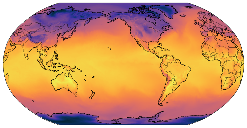
Last but not least we visualize the 2m air temperature (tas) from this ICON dataset.
worldmap(ds.tas.isel(time=0), cmap=cmocean.cm.thermal)